User:Yak90

Different texts (and even different parts of this article) adopt slightly different definitions for the negative binomial distribution. They can be distinguished by whether the support starts at k = 0 or at k = r, whether p denotes the probability of a success or of a failure, and whether r represents success or failure, so identifying the specific parametrization used is crucial in any given text.
Probability mass function The orange line represents the mean, which is equal to 10 in each of these plots; the green line shows the standard deviation.
Notation	$\mathrm {NB} (r,\,p)$
Parameters	r > 0 — number of successes until the experiment is stopped (integer, but the definition can also be extended to reals) p ∈ [0,1] — success probability in each experiment (real)
Support	k ∈ { 0, 1, 2, 3, … } — number of failures
PMF	$k\mapsto {k+r-1 \choose k}\cdot (1-p)^{k}p^{r},$ involving a binomial coefficient
CDF	$k\mapsto I_{p}(r,\,k+1),$ the regularized incomplete beta function
Mean	${\frac {r(1-p)}{p}}$
Mode	${\begin{cases}\left\lfloor {\frac {(r-1)(1-p)}{p}}\right\rfloor &{\text{if }}r>1\\0&{\text{if }}r\leq 1\end{cases}}$
Variance	${\frac {r(1-p)}{p^{2}}}$
Skewness	${\frac {2-p}{\sqrt {(1-p)r}}}$
Excess kurtosis	${\frac {6}{r}}+{\frac {p^{2}}{(1-p)r}}$
MGF	${\biggl (}{\frac {p}{1-(1-p)e^{t}}}{\biggr )}^{\!r}{\text{ for }}t<-\log(1-p)$
CF	${\biggl (}{\frac {p}{1-(1-p)e^{i\,t}}}{\biggr )}^{\!r}{\text{ with }}t\in \mathbb {R}$
PGF	${\biggl (}{\frac {p}{1-(1-p)z}}{\biggr )}^{\!r}{\text{ for }}|z|<{\frac {1}{p}}$
Fisher information	${\frac {r}{p^{2}(1-p)}}$
Method of moments	$r={\frac {E[X]^{2}}{V[X]-E[X]}}$ $p={\frac {E[X]}{V[X]}}$

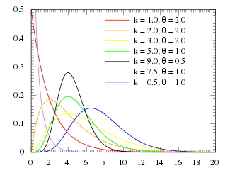
The negative binomial distribution also arises as a continuous mixture of Poisson distributions (i.e. a compound probability distribution) where the mixing distribution of the Poisson rate is a gamma distribution. That is, we can view the negative binomial as a Poisson(λ) distribution, where λ is itself a random variable, distributed as a gamma distribution with shape = r and scale θ = p/(1 − p) or correspondingly rate β = (1 − p)/p.

Different texts adopt slightly different definitions for the negative binomial distribution. They can be distinguished by whether the support starts at k = 0 or at k = r, whether p denotes the probability of a success or of a failure, and whether r represents success or failure, so it is crucial to identify the specific parametrization used in any given text.
Probability mass function The orange line represents the mean, which is equal to 10 in each of these plots; the green line shows the standard deviation.
Notation	$\mathrm {NB2} (\mu ,\,\phi )$
Parameters	r > 0 — number of failures until the experiment is stopped (integer, but the definition can also be extended to reals) p ∈ (0,1) — success probability in each experiment (real)
Support	k ∈ { 0, 1, 2, 3, … } — number of successes
PMF	${k+r-1 \choose k}\cdot (1-p)^{r}p^{k},$ involving a binomial coefficient
CDF	$1-I_{p}(k+1,\,r),$ the regularized incomplete beta function
Mean	$\mu$
Mode	${\begin{cases}{\big \lfloor }{\frac {p(r-1)}{1-p}}{\big \rfloor }&{\text{if}}\ r>1\\0&{\text{if}}\ r\leq 1\end{cases}}$
Variance	$\mu +{\frac {\mu ^{2}}{\phi }}$
Skewness	${\frac {1+p}{\sqrt {pr}}}$
Excess kurtosis	${\frac {6}{r}}+{\frac {(1-p)^{2}}{pr}}$
MGF	${\biggl (}{\frac {1-p}{1-pe^{t}}}{\biggr )}^{\!r}{\text{ for }}t<-\log p$
CF	${\biggl (}{\frac {1-p}{1-pe^{i\,t}}}{\biggr )}^{\!r}{\text{ with }}t\in \mathbb {R}$
PGF	${\biggl (}{\frac {1-p}{1-pz}}{\biggr )}^{\!r}{\text{ for }}|z|<{\frac {1}{p}}$
Fisher information	${\frac {r}{(1-p)^{2}p}}$

Gamma

Probability density function
Cumulative distribution function
Parameters	k > 0 shape θ > 0 scale	α > 0 shape β > 0 rate
Support	$x\in (0,\infty )$	$x\in (0,\infty )$
PDF	${\frac {1}{\Gamma (k)\theta ^{k}}}x^{k-1}e^{-{\frac {x}{\theta }}}$	${\frac {\beta ^{\alpha }}{\Gamma (\alpha )}}x^{\alpha -1}e^{-\beta x}$
CDF	${\frac {1}{\Gamma (k)}}\gamma \left(k,{\frac {x}{\theta }}\right)$	${\frac {1}{\Gamma (\alpha )}}\gamma (\alpha ,\beta x)$
Mean	$\operatorname {E} [X]=k\theta$	$\operatorname {E} [X]={\frac {\alpha }{\beta }}$
Median	No simple closed form	No simple closed form
Mode	$(k-1)\theta {\text{ for }}k\geq 1$	${\frac {\alpha -1}{\beta }}{\text{ for }}\alpha \geq 1$
Variance	$\operatorname {Var} (X)=k\theta ^{2}$	$\operatorname {Var} (X)={\frac {\alpha }{\beta ^{2}}}$
Skewness	${\frac {2}{\sqrt {k}}}$	${\frac {2}{\sqrt {\alpha }}}$
Excess kurtosis	${\frac {6}{k}}$	${\frac {6}{\alpha }}$
Entropy	${\begin{aligned}k&+\ln \theta +\ln \Gamma (k)\\&+(1-k)\psi (k)\end{aligned}}$	${\begin{aligned}\alpha &-\ln \beta +\ln \Gamma (\alpha )\\&+(1-\alpha )\psi (\alpha )\end{aligned}}$
MGF	$(1-\theta t)^{-k}{\text{ for }}t<{\frac {1}{\theta }}$	$\left(1-{\frac {t}{\beta }}\right)^{-\alpha }{\text{ for }}t<\beta$
CF	$(1-\theta it)^{-k}$	$\left(1-{\frac {it}{\beta }}\right)^{-\alpha }$