User:Rojasmar/sandbox

A visual representation of the Glatzmaier model before dipole reversal

Expanding "Numerical modeling" section of Dynamo theory

*quotations are all from Dynamo theory wiki article and will be removed once moved there

A visual representation of the Glatzmaier model during dipole reversal

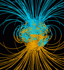
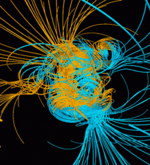
Broadly, models of dynamo attempt to produce magnetic fields consistent with observed data given certain conditions and equations as mentioned in the sections above. Implementing the magnetohydrodynamic equations successfully was of particular significance because they pushed dynamo models to self-consistency. Though geodynamo models are especially prevalent, dynamo models are not necessarily restricted to the geodynamo; solar and general dynamo models are also of interest. Studying dynamo models has utility in the field of geophysics as doing so can identify how various mechanisms form magnetic fields like those produced by astrophysical bodies like Earth and how they cause magnetic fields to exhibit certain features, such as pole reversals.

The equations used in numerical models of dynamo are highly complex. "For decades, theorists were confined" to two dimensional "kinematic dynamo models described above, in which the fluid motion is chosen in advance and the effect on the magnetic field calculated." The progression from linear to nonlinear, three dimensional models of dynamo was largely hindered by the search for solutions to magnetohydrodynamic equations, which eliminate the need for many of the assumptions made in kinematic models and allow self-consistency.

A visual representation of the Glatzmaier model after dipole reversal

"The first self-consistent dynamo models, ones that determine both the fluid motions and the magnetic field" through magnetohydrodynamic equations", were developed by two groups in 1995, one in Japan and one in the United States. The latter" was made as a model with regards to the geodynamo and "received significant attention because it successfully reproduced some of the characteristics of the Earth's field." Following this breakthrough, there was a large swell in development of reasonable, three dimensional dynamo models.

Though many self-consistent models now exist, there are significant differences among the models, both in the results they produce and the way they were developed. Given the complexity of developing a geodynamo model, there are many places where discrepancies can occur such as when making assumptions involving the mechanisms that provide energy for the dynamo, when choosing values for parameters used in equations, or when normalizing equations. In spite of the many differences that may occur, most models have shared features like clear axial dipoles. In many of these models, phenomena like secular variation and geomagnetic polarity reversals have also been successfully recreated.

Observations

Many observations can be made from dynamo models. Models can be used to estimate how magnetic fields vary with time and can be compared to observed paleomagnetic data to find similarities between the model and the Earth. Due to the uncertainty of paleomagnetic observations, however, comparisons may not be entirely valid or useful. Simplified geodynamo models have shown relationships between the dynamo number (determined by variance in rotational rates in the outer core and mirror-asymmetric convection (e.g. when convection favors one direction in the north and the other in the south)) and magnetic pole reversals as well as found similarities between the geodynamo and the Sun's dynamo. In many models, it appears that magnetic fields have somewhat random magnitudes that follow a normal trend that average to zero. In addition to these observations, general observations about the mechanisms powering the geodynamo can be made based on how accurately the model reflects actual data collected from Earth.

Modern Modelling

The complexity of dynamo modelling is so great that models of the geodynamo are limited by the current power of supercomputers, particularly because calculating the Ekman and Rayleigh number of the outer core is extremely difficult and requires a vast number of computations.

Many improvements have been proposed in dynamo modelling since the self-consistent breakthrough in 1995. One suggestion in studying the complex magnetic field changes is applying spectral analysis methods to simplify computations.(potentially going to be excluded or more improvements will be added). Ultimately, until considerable improvements in computer power are made, the methods for computing realistic dynamo models will have to be made more efficient, so making improvements in methods for computing the model is of high importance for the advancement of numerical dynamo modelling.

References

[edit]- ^ a b c d e Kono, Masaru; Roberts, Paul H. (2002). "Recent Geodynamo Simulations and Observations of the Geomagnetic Field". Reviews of Geophysics. 40 (4): 4–1–4-53. doi:10.1029/2000RG000102. ISSN 1944-9208.
- ^ Yushkov, E. V.; Sokoloff, D. D. (2018-07-01). "Geomagnetic Reversals and Dynamo Bursts in a Simple Geodynamo Model". Izvestiya, Physics of the Solid Earth. 54 (4): 652–657. doi:10.1134/S1069351318040122. ISSN 1555-6506.
- ^ Avery, Margaret S.; Constable, Catherine G.; Davies, Christopher J.; Gubbins, David (2019-01-01). "Spectral methods for analyzing energy balances in geodynamo simulations". Physics of the Earth and Planetary Interiors. 286: 127–137. doi:10.1016/j.pepi.2018.10.002. ISSN 0031-9201.