t-J model

2D Hubbard model. The t-J model is the Hubbard model for U >> t

In solid-state physics, the t-J model is a model first derived by Józef Spałek to explain antiferromagnetic properties of Mott insulators, taking into account experimental results about the strength of electron-electron repulsion in these materials.

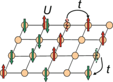
The material is modelled as a lattice with atoms in the sites with conduction electrons (or holes) moving between them, like in the Hubbard model. Unlike the Hubbard model, the electrons are strongly-correlated, meaning the electrons are sensitive to reciprocal coulombic repulsion, and so are less likely to occupy lattice sites already occupied by another electron. In the basic Hubbard model, the repulsion, indicated by U, can be small or even zero, and electrons are more free to jump (hopping, parametrized by t as transfer or tunnel) from one site to another. In the t-J model, instead of U, there is the parameter J, function of the ratio t/U.

Like the Hubbard model, it is a prospective microscopic theory of high temperature superconductivity in cuprate superconductors which arise from doped antiferromagnets, particularly in the case where the lattice considered is the two-dimensional lattice. Cuprate superconductors are currently (as of 2024) the superconductors with the highest known superconducting transition temperature at ambient pressure, but there is no consensus on the microscopic theory responsible for their superconducting transition.

The Hamiltonian

In quantum physics, system's models are usually based on the Hamiltonian operator ${\hat {H}}$, corresponding to the total energy of that system, including both kinetic energy and potential energy.

The t-J Hamiltonian can be derived from the ${\hat {H}}$ of the Hubbard model using the Schrieffer–Wolff transformation, with the transformation generator depending on t/U and excluding the possibility for electrons to doubly occupy a lattice's site, which results in:

${\hat {H}}=-t\sum _{\langle ij\rangle ,\sigma }\left(c_{i\sigma }^{\dagger }c_{j\sigma }+\mathrm {h.c.} \right)+J\sum _{\langle ij\rangle }\left(\mathbf {S} _{i}\cdot \mathbf {S} _{j}-{\frac {n_{i}n_{j}}{4}}\right)+O(t^{3}/U^{2})$

where the term in t corresponds to the kinetic energy and is equal to the one in the Hubbard model. The second one is the potential energy approximated at the second order, because this is an approximation of the Hubbard model in the limit U >> t developed in power of t. Terms at higher order can be added.

The parameters are:

• Σ⟨ij⟩ is the sum over nearest-neighbor sites i and j, for all sites, typically on a two-dimensional square lattice,
• c^†
  _iσ, c
  _iσ are the fermionic creation and annihilation operators at site i,
• σ is the spin polarization,
• t is the hopping integral,
• J is the antiferromagnetic exchange coupling, J = ⁠4t²/U⁠,
• U is the on-site coulombic repulsion, that must satisfy the condition for U >> t,
• n_i = Σσc^†
  _iσc
  _iσ is the particle number at site i and can be maximum 1, so that double occupancy is forbidden (in the Hubbard model is possible),
• S_i and S_j are the spins on sites i and j,
• h. c. stands for Hermitian conjugate,

If n_i = 1, that is when in the ground state, there is just one electron per lattice's site (half-filling), the model reduces to the Heisenberg model and the ground state reproduce a dielectric antiferromagnets (Mott insulator).

The model can be further extended considering also the next-nearest-neighbor sites and the chemical potential to set the ground state in function of the total number of particles:

${\mathcal {\hat {H}}}=t_{1}\sum \limits _{\langle i,j\rangle }\left(c_{i\sigma }^{\dagger }c_{j\sigma }+\mathrm {h.c.} \right)\ +\ t_{2}\sum \limits _{\langle \langle i,j\rangle \rangle }\left(c_{i\sigma }^{\dagger }c_{j\sigma }+\mathrm {h.c.} \right)\ +\ J\sum \limits _{\langle i,j\rangle }\left(\mathbf {S} _{i}\cdot \mathbf {S} _{j}-{\frac {n_{i}n_{j}}{4}}\right)-\ \mu \sum \limits _{i}n_{i},$

where ⟨...⟩ and ⟨⟨...⟩⟩ denote the nearest and next-nearest neighbors, respectively, with two different values for the hopping integral (t₁ and t₂) and μ is the chemical potential.

Further reading

• Fazekas, Patrik (1999). Lectures on Correlation and Magnetism. Series in Modern Condensed Matter Physics: Volume 5. Vol. 5. World Scientific. p. 199. doi:10.1142/2945. ISBN 978-981-4499-62-0.
• Spałek, Józef (2007). "t-J model then and now: A personal perspective from the pioneering times". Acta Phys. Pol. A. 111 (4): 409–424. arXiv:0706.4236. Bibcode:2007AcPPA.111..409S. doi:10.12693/APhysPolA.111.409. S2CID 53117123.
• Dr Mitchell, Electron interactions and the Hubbard model, retrieved 2022-08-29

References

[edit]- ^ a b Chao, K. A.; Spałek, J.; Oleś, A. M. (1978-10-01). "Canonical perturbation expansion of the Hubbard model". Physical Review B. 18 (7): 3453–3464. Bibcode:1978PhRvB..18.3453C. doi:10.1103/PhysRevB.18.3453.
- ^ Anderson, P. W. (1959-07-01). "New Approach to the Theory of Superexchange Interactions". Physical Review. 115 (1): 2–13. Bibcode:1959PhRv..115....2A. doi:10.1103/PhysRev.115.2.
- ^ Nagaoka, Yosuke (1966-07-08). "Ferromagnetism in a Narrow, Almost Half-Filled s Band". Physical Review. 147 (1): 392–405. Bibcode:1966PhRv..147..392N. doi:10.1103/PhysRev.147.392.
- ^ Spalek, Jozef (2007-06-28). "t-J model then and now: A personal perspective from the pioneering times". Acta Physica Polonica A. 111 (4): 409. arXiv:0706.4236. Bibcode:2007AcPPA.111..409S. doi:10.12693/APhysPolA.111.409. S2CID 53117123.
- ^ Rømer, Astrid T.; Maier, Thomas A.; Kreisel, Andreas; Eremin, Ilya; Hirschfeld, P. J.; Andersen, Brian M. (2020-01-31). "Pairing in the two-dimensional Hubbard model from weak to strong coupling". Physical Review Research. 2 (1): 013108. arXiv:1909.00627. Bibcode:2020PhRvR...2a3108R. doi:10.1103/PhysRevResearch.2.013108. S2CID 202540002.
- ^ This is done using a projector quantum operator that project on the subspace where fermionic operators can not add an electron on a site already occupied (see next note)
- ^ Eckle, Hans-Peter (2019). "8.8.1 From the Hubbard to the t–J model: non-half filled band case" (PDF). Models of Quantum Matter. Oxford University Press. ISBN 9780199678839.
- ^ Izyumov, Yu. A.; Chashchin, N. I. (1998). "tJ -model in terms of equations with variational derivatives". Condensed Matter Physics. 1 (1): 41–56. Bibcode:1998CMPh....1...41I. doi:10.5488/CMP.1.1.41. S2CID 11254082.
- ^ Karchev, Naoum (1998). "Generalized CP1 model from the t1-t2-J model". Phys. Rev. B. 57 (17): 10913. arXiv:cond-mat/9706105. Bibcode:1998PhRvB..5710913K. doi:10.1103/PhysRevB.57.10913. S2CID 12865671.
- ^ Yanagisawa, Takashi (2008-02-12). "Phase diagram of thet–U2Hamiltonian of the weak coupling Hubbard model". New Journal of Physics. 10 (2): 023014. arXiv:0803.1739. Bibcode:2008NJPh...10b3014Y. doi:10.1088/1367-2630/10/2/023014. ISSN 1367-2630. S2CID 55405863.