Kruskal–Wallis test

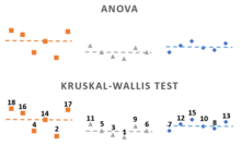
The Kruskal–Wallis test by ranks, Kruskal–Wallis test (named after William Kruskal and W. Allen Wallis), or one-way ANOVA on ranks is a non-parametric statistical test for testing whether samples originate from the same distribution.[1][2][3] It is used for comparing two or more independent samples of equal or different sample sizes. It extends the Mann–Whitney U test, which is used for comparing only two groups. The parametric equivalent of the Kruskal–Wallis test is the one-way analysis of variance (ANOVA).
A significant Kruskal–Wallis test indicates that at least one sample stochastically dominates one other sample. The test does not identify where this stochastic dominance occurs or for how many pairs of groups stochastic dominance obtains. For analyzing the specific sample pairs for stochastic dominance, Dunn's test,[4] pairwise Mann–Whitney tests with Bonferroni correction,[5] or the more powerful but less well known Conover–Iman test[5] are sometimes used.
It is supposed that the treatments significantly affect the response level and then there is an order among the treatments: one tends to give the lowest response, another gives the next lowest response is second, and so forth.[6] Since it is a nonparametric method, the Kruskal–Wallis test does not assume a normal distribution of the residuals, unlike the analogous one-way analysis of variance. If the researcher can make the assumptions of an identically shaped and scaled distribution for all groups, except for any difference in medians, then the null hypothesis is that the medians of all groups are equal, and the alternative hypothesis is that at least one population median of one group is different from the population median of at least one other group. Otherwise, it is impossible to say, whether the rejection of the null hypothesis comes from the shift in locations or group dispersions. This is the same issue that happens also with the Mann-Whitney test.[7][8][9] If the data contains potential outliers, if the population distributions have heavy tails, or if the population distributions are significantly skewed, the Kruskal-Wallis test is more powerful at detecting differences among treatments than ANOVA F-test. On the other hand, if the population distributions are normal or are light-tailed and symmetric, then ANOVA F-test will generally have greater power which is the probability of rejecting the null hypothesis when it indeed should be rejected.[10][11]
Method
[edit]
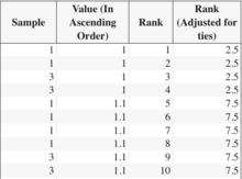
- Rank all data from all groups together; i.e., rank the data from 1 to N ignoring group membership. Assign any tied values the average of the ranks they would have received had they not been tied.
- The test statistic is given by
- where
- is the total number of observations across all groups
- is the number of groups
- is the number of observations in group
- is the rank (among all observations) of observation from group
- is the average rank of all observations in group
- is the average of all the .
- If the data contain no ties, the denominator of the expression for is exactly and . Thus
The last formula contains only the squares of the average ranks.
- A correction for ties if using the short-cut formula described in the previous point can be made by dividing by , where is the number of groupings of different tied ranks, and is the number of tied values within group that are tied at a particular value. This correction usually makes little difference in the value of unless there are a large number of ties.
- When performing multiple sample comparisons, the type I error tends to become inflated. Therefore, the Bonferroni procedure is used to adjust the significance level, that is, , where is the adjusted significance level, is the initial significance level, and is the number of contrasts.[12]
- Finally, the decision to reject or accept the null hypothesis is made by comparing to a critical value (obtained from a table or software) for a given significance or alpha level. If is bigger than , the null hypothesis is rejected. If possible (no ties, sample not too big) one should compare to the critical value obtained from the exact distribution of . Otherwise, the distribution of H can be approximated by a chi-squared distribution with degrees of freedom. If some values are small (i.e., less than 5) the exact probability distribution of can be quite different from this chi-squared distribution. If a table of the chi-squared probability distribution is available, the critical value of chi-squared, , can be found by entering the table at degrees of freedom and looking under the desired significance or alpha level.[13]
- If the statistic is not significant, there is no evidence of stochastic dominance among the samples. However, if the test is significant then at least one sample stochastically dominates another sample. Then, a researcher might use sample contrasts between individual sample pairs, or post hoc tests using Dunn's test, which (1) properly employs the same rankings as the Kruskal–Wallis test, and (2) properly employs the pooled variance implied by the null hypothesis of the Kruskal–Wallis test in order to determine which of the sample pairs are significantly different.[4] When performing multiple sample contrasts or tests, the Type I error rate tends to become inflated, raising concerns about multiple comparisons.
Exact probability tables
[edit]A large amount of computing resources is required to compute exact probabilities for the Kruskal–Wallis test. Existing software only provides exact probabilities for sample sizes of less than about 30 participants. These software programs rely on the asymptotic approximation for larger sample sizes. Exact probability values for larger sample sizes are available. Spurrier (2003) published exact probability tables for samples as large as 45 participants.[14] Meyer and Seaman (2006) produced exact probability distributions for samples as large as 105 participants.[15]
Exact distribution of H
[edit]Choi et al.[16] made a review of two methods that had been developed to compute the exact distribution of , proposed a new one, and compared the exact distribution to its chi-squared approximation.
Example
[edit]Test for differences in ozone levels by month
[edit]The following example uses data from Chambers et al.[17]
on daily readings of ozone for May 1 to September 30, 1973, in New York City. The data are in the R data set airquality, and the analysis is included in the documentation for the R function kruskal.test. Boxplots of ozone values by month are shown in the figure.
The Kruskal-Wallis test finds a significant difference (p = 6.901e-06) indicating that ozone differs among the 5 months.
kruskal.test(Ozone ~ Month, data = airquality)

	Kruskal-Wallis rank sum test

data:  Ozone by Month
Kruskal-Wallis chi-squared = 29.267, df = 4, p-value = 6.901e-06
To determine which months differ, post-hoc tests may be performed using a Wilcoxon test for each pair of months, with a Bonferroni (or other) correction for multiple hypothesis testing.
pairwise.wilcox.test(airquality$Ozone, airquality$Month, p.adjust.method = "bonferroni")

	Pairwise comparisons using Wilcoxon rank sum test

data:  airquality$Ozone and airquality$Month

  5      6      7      8
6 1.0000 -      -      -
7 0.0003 0.1414 -      -
8 0.0012 0.2591 1.0000 -
9 1.0000 1.0000 0.0074 0.0325

P value adjustment method: bonferroni
The post-hoc tests indicate that, after Bonferroni correction for multiple testing, the following differences are significant (adjusted p < 0.05).
- Month 5 vs Months 7 and 8
- Month 9 vs Months 7 and 8
Implementation
[edit]The Kruskal-Wallis test can be implemented in many programming tools and languages. We list here only the open source free software packages:
- In Python's SciPy package, the function
scipy.stats.kruskalcan return the test result and p-value.[18] - R base-package has an implement of this test using
kruskal.test.[19] - Java has the implement provided by provided by Apache Commons.[20]
- In Julia, the package
HypothesisTests.jlhas the functionKruskalWallisTest(groups::AbstractVector{<:Real}...)to compute the p-value.[21]
See also
[edit]- One-way ANOVA
- Mann–Whitney U tests
- Bonferroni test
- Friedman test
- Jonckheere's trend test
- Mood's Median test
References
[edit]- ^ Kruskal; Wallis (1952). "Use of ranks in one-criterion variance analysis". Journal of the American Statistical Association. 47 (260): 583–621. doi:10.1080/01621459.1952.10483441.
- ^ Corder, Gregory W.; Foreman, Dale I. (2009). Nonparametric Statistics for Non-Statisticians. Hoboken: John Wiley & Sons. pp. 99–105. ISBN 9780470454619.
- ^ Siegel; Castellan (1988). Nonparametric Statistics for the Behavioral Sciences (Second ed.). New York: McGraw–Hill. ISBN 0070573573.
- ^ a b Dunn, Olive Jean (1964). "Multiple comparisons using rank sums". Technometrics. 6 (3): 241–252. doi:10.2307/1266041.
- ^ a b Conover, W. Jay; Iman, Ronald L. (1979). "On multiple-comparisons procedures" (PDF) (Report). Los Alamos Scientific Laboratory. Retrieved 2016-10-28.
- ^ Lehmann, E. L., & D'Abrera, H. J. (1975). Nonparametrics: Statistical methods based on ranks. Holden-Day.
- ^ Divine; Norton; Barón; Juarez-Colunga (2018). "The Wilcoxon–Mann–Whitney Procedure Fails as a Test of Medians". The American Statistician. doi:10.1080/00031305.2017.1305291.
- ^ Hart (2001). "Mann-Whitney test is not just a test of medians: differences in spread can be important". BMJ. doi:10.1136/bmj.323.7309.391.
- ^ Bruin (2006). "FAQ: Why is the Mann-Whitney significant when the medians are equal?". UCLA: Statistical Consulting Group.
- ^ Higgins, James J.; Jeffrey Higgins, James (2004). An introduction to modern nonparametric statistics. Duxbury advanced series. Pacific Gove, CA: Brooks-Cole; Thomson Learning. ISBN 978-0-534-38775-4.
- ^ Berger, Paul D.; Maurer, Robert E.; Celli, Giovana B. (2018). Experimental Design. Cham: Springer International Publishing. doi:10.1007/978-3-319-64583-4. ISBN 978-3-319-64582-7.
- ^ Corder, G.W. & Foreman, D.I. (2010). Nonparametric Statistics for Non-statisticians: A Step-by-Step Approach. Hoboken, NJ: Wiley.
- ^ Montgomery, Douglas C.; Runger, George C. (2018). Applied statistics and probability for engineers. EMEA edition (Seventh ed.). Hoboken, NJ: Wiley. ISBN 978-1-119-40036-3.
- ^ Spurrier, J. D. (2003). "On the null distribution of the Kruskal–Wallis statistic". Journal of Nonparametric Statistics. 15 (6): 685–691. doi:10.1080/10485250310001634719.
- ^ Meyer; Seaman (April 2006). "Expanded tables of critical values for the Kruskal–Wallis H statistic". Paper presented at the annual meeting of the American Educational Research Association, San Francisco. Critical value tables and exact probabilities from Meyer and Seaman are available for download at http://faculty.virginia.edu/kruskal-wallis/ Archived 2018-10-17 at the Wayback Machine. A paper describing their work may also be found there.
- ^ Won Choi, Jae Won Lee, Myung-Hoe Huh, and Seung-Ho Kang (2003). "An Algorithm for Computing the Exact Distribution of the Kruskal–Wallis Test". Communications in Statistics - Simulation and Computation (32, number 4): 1029–1040. doi:10.1081/SAC-120023876.
{{cite journal}}: CS1 maint: multiple names: authors list (link) - ^ John M. Chambers, William S. Cleveland, Beat Kleiner, and Paul A. Tukey (1983). Graphical Methods for Data Analysis. Belmont, Calif: Wadsworth International Group, Duxbury Press. ISBN 053498052X.
{{cite book}}: CS1 maint: multiple names: authors list (link) - ^ "scipy.stats.kruskal — SciPy v1.11.4 Manual". docs.scipy.org. Retrieved 2023-12-06.
- ^ "kruskal.test function - RDocumentation". www.rdocumentation.org. Retrieved 2023-12-06.
- ^ "Math – The Commons Math User Guide - Statistics". commons.apache.org. Retrieved 2023-12-06.
- ^ "Nonparametric tests · HypothesisTests.jl". juliastats.org. Retrieved 2023-12-06.
Further reading
[edit]- Daniel, Wayne W. (1990). "Kruskal–Wallis one-way analysis of variance by ranks". Applied Nonparametric Statistics (2nd ed.). Boston: PWS-Kent. pp. 226–234. ISBN 0-534-91976-6.


