Kelly criterion

In probability theory, the Kelly criterion (or Kelly strategy or Kelly bet) is a formula for sizing a sequence of bets by maximizing the long-term expected value of the logarithm of wealth, which is equivalent to maximizing the long-term expected geometric growth rate. John Larry Kelly Jr., a researcher at Bell Labs, described the criterion in 1956.[1]
The practical use of the formula has been demonstrated for gambling,[2][3] and the same idea was used to explain diversification in investment management.[4] In the 2000s, Kelly-style analysis became a part of mainstream investment theory[5] and the claim has been made that well-known successful investors including Warren Buffett[6] and Bill Gross[7] use Kelly methods.[8] Also see intertemporal portfolio choice. It is also the standard replacement of statistical power in anytime-valid statistical tests and confidence intervals, based on e-values and e-processes.
Kelly criterion for binary return rates
[edit]In a system where the return on an investment or a bet is binary, so an interested party either wins or loses a fixed percentage of their bet, the expected growth rate coefficient yields a very specific solution for an optimal betting percentage.
Gambling Formula
[edit]Where losing the bet involves losing the entire wager, the Kelly bet is:
where:
- is the fraction of the current bankroll to wager.
- is the probability of a win.
- is the probability of a loss.
- is the proportion of the bet gained with a win. E.g., if betting $10 on a 2-to-1 odds bet (upon win you are returned $30, winning you $20), then .

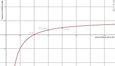
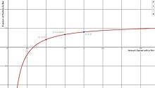
The figure plots the amount gained with a win on the x-axis against the fraction of portfolio to bet on the y-axis. This figure assumes p=0.5 (that the probability of both a win and a loss is 50%). If the amount gained with a win is 1, then the Kelly betting amount is $0, which makes sense in a fair bet with no expected gain.
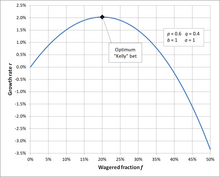
As an example, if a gamble has a 60% chance of winning (, ), and the gambler receives 1-to-1 odds on a winning bet (), then to maximize the long-run growth rate of the bankroll, the gambler should bet 20% of the bankroll at each opportunity ().


If the gambler has zero edge (i.e., if ), then the criterion recommends the gambler bet nothing.
If the edge is negative (), the formula gives a negative result, indicating that the gambler should take the other side of the bet.
Investment formula
[edit]A more general form of the Kelly formula allows for partial losses, which is relevant for investments:[9]: 7
where:
- is the fraction of the assets to apply to the security.
- is the probability that the investment increases in value.
- is the probability that the investment decreases in value ().
- is the fraction that is gained in a positive outcome.[9]: 7 If the security price rises 10%, then .
- is the fraction that is lost in a negative outcome.[9]: 7 If the security price falls 10%, then
Note that the Kelly criterion is perfectly valid only for fully known outcome probabilities, which is almost never the case with investments. In addition, risk-averse strategies invest less than the full Kelly fraction.
The general form can be rewritten as follows
where:
- is the win-loss probability (WLP) ratio, which is the ratio of winning to losing bets.
- is the win-loss ratio (WLR) of bet outcomes, which is the winning skew.
It is clear that, at least, one of the factors or needs to be larger than 1 for having an edge (so ). It is even possible that the win-loss probability ratio is unfavorable , but one has an edge as long as .
The Kelly formula can easily result in a fraction higher than 1, such as with losing size (see the above expression with factors of and ). This happens somewhat counterintuitively, because the Kelly fraction formula compensates for a small losing size with a larger bet. However, in most real situations, there is high uncertainty about all parameters entering the Kelly formula. In the case of a Kelly fraction higher than 1, it is theoretically advantageous to use leverage to purchase additional securities on margin.
Betting example – behavioural experiment
[edit]In a study, each participant was given $25 and asked to place even-money bets on a coin that would land heads 60% of the time. Participants had 30 minutes to play, so could place about 300 bets, and the prizes were capped at $250. But the behavior of the test subjects was far from optimal:
Remarkably, 28% of the participants went bust, and the average payout was just $91. Only 21% of the participants reached the maximum. 18 of the 61 participants bet everything on one toss, while two-thirds gambled on tails at some stage in the experiment.[10][11]
Using the Kelly criterion and based on the odds in the experiment (ignoring the cap of $250 and the finite duration of the test), the right approach would be to bet 20% of one's bankroll on each toss of the coin, which works out to a 2.034% average gain each round. This is a geometric mean, not the arithmetic rate of 4% (r = 0.2 x (0.6 - 0.4) = 0.04). The theoretical expected wealth after 300 rounds works out to $10,505 () if it were not capped.
In this particular game, because of the cap, a strategy of betting only 12% of the pot on each toss would have even better results (a 95% probability of reaching the cap and an average payout of $242.03).
Proof
[edit]Heuristic proofs of the Kelly criterion are straightforward.[12] The Kelly criterion maximizes the expected value of the logarithm of wealth (the expectation value of a function is given by the sum, over all possible outcomes, of the probability of each particular outcome multiplied by the value of the function in the event of that outcome). We start with 1 unit of wealth and bet a fraction of that wealth on an outcome that occurs with probability and offers odds of . The probability of winning is , and in that case the resulting wealth is equal to . The probability of losing is and the odds of a negative outcome is . In that case the resulting wealth is equal to . Therefore, the expected geometric growth rate is:
We want to find the maximum r of this curve (as a function of f), which involves finding the derivative of the equation. This is more easily accomplished by taking the logarithm of each side first; because the logarithm is monotonic, it does not change the locations of function extrema. The resulting equation is:
with denoting logarithmic wealth growth. To find the value of for which the growth rate is maximized, denoted as , we differentiate the above expression and set this equal to zero. This gives:
Rearranging this equation to solve for the value of gives the Kelly criterion:
Notice that this expression reduces to the simple gambling formula when , when a loss results in full loss of the wager.
Kelly criterion for non-binary return rates
[edit]If the return rates on an investment or a bet are continuous in nature the optimal growth rate coefficient must take all possible events into account.
Application to the stock market
[edit]In mathematical finance, if security weights maximize the expected geometric growth rate (which is equivalent to maximizing log wealth), then a portfolio is growth optimal.
The Kelly Criterion shows that for a given volatile security this is satisfied when
where is the fraction of available capital invested that maximizes the expected geometric growth rate, is the expected growth rate coefficient, is the variance of the growth rate coefficient and is the risk-free rate of return. Note that a symmetric probability density function was assumed here.
Computations of growth optimal portfolios can suffer tremendous garbage in, garbage out problems. For example, the cases below take as given the expected return and covariance structure of assets, but these parameters are at best estimates or models that have significant uncertainty. If portfolio weights are largely a function of estimation errors, then Ex-post performance of a growth-optimal portfolio may differ fantastically from the ex-ante prediction. Parameter uncertainty and estimation errors are a large topic in portfolio theory. An approach to counteract the unknown risk is to invest less than the Kelly criterion.
Rough estimates are still useful. If we take excess return 4% and volatility 16%, then yearly Sharpe ratio and Kelly ratio are calculated to be 25% and 150%. Daily Sharpe ratio and Kelly ratio are 1.7% and 150%. Sharpe ratio implies daily win probability of p=(50% + 1.7%/4), where we assumed that probability bandwidth is . Now we can apply discrete Kelly formula for above with , and we get another rough estimate for Kelly fraction . Both of these estimates of Kelly fraction appear quite reasonable, yet a prudent approach suggest a further multiplication of Kelly ratio by 50% (i.e. half-Kelly).
A detailed paper by Edward O. Thorp and a co-author estimates Kelly fraction to be 117% for the American stock market SP500 index. [13] Significant downside tail-risk for equity markets is another reason[14] to reduce Kelly fraction from naive estimate (for instance, to reduce to half-Kelly).
Proof
[edit]A rigorous and general proof can be found in Kelly's original paper[1] or in some of the other references listed below. Some corrections have been published.[15] We give the following non-rigorous argument for the case with (a 50:50 "even money" bet) to show the general idea and provide some insights.[1] When , a Kelly bettor bets times their initial wealth , as shown above. If they win, they have after one bet. If they lose, they have . Suppose they make bets like this, and win times out of this series of bets. The resulting wealth will be:
The ordering of the wins and losses does not affect the resulting wealth. Suppose another bettor bets a different amount, for some value of (where may be positive or negative). They will have after a win and after a loss. After the same series of wins and losses as the Kelly bettor, they will have:
Take the derivative of this with respect to and get:
The function is maximized when this derivative is equal to zero, which occurs at:
which implies that
but the proportion of winning bets will eventually converge to:
according to the weak law of large numbers. So in the long run, final wealth is maximized by setting to zero, which means following the Kelly strategy. This illustrates that Kelly has both a deterministic and a stochastic component. If one knows K and N and wishes to pick a constant fraction of wealth to bet each time (otherwise one could cheat and, for example, bet zero after the Kth win knowing that the rest of the bets will lose), one will end up with the most money if one bets:
each time. This is true whether is small or large. The "long run" part of Kelly is necessary because K is not known in advance, just that as gets large, will approach . Someone who bets more than Kelly can do better if for a stretch; someone who bets less than Kelly can do better if for a stretch, but in the long run, Kelly always wins. The heuristic proof for the general case proceeds as follows.[citation needed] In a single trial, if one invests the fraction of their capital, if the strategy succeeds, the capital at the end of the trial increases by the factor , and, likewise, if the strategy fails, the capital is decreased by the factor . Thus at the end of trials (with successes and failures), the starting capital of $1 yields
Maximizing , and consequently , with respect to leads to the desired result
Edward O. Thorp provided a more detailed discussion of this formula for the general case.[9] There, it can be seen that the substitution of for the ratio of the number of "successes" to the number of trials implies that the number of trials must be very large, since is defined as the limit of this ratio as the number of trials goes to infinity. In brief, betting each time will likely maximize the wealth growth rate only in the case where the number of trials is very large, and and are the same for each trial. In practice, this is a matter of playing the same game over and over, where the probability of winning and the payoff odds are always the same. In the heuristic proof above, successes and failures are highly likely only for very large .
Multiple outcomes
[edit]Kelly's criterion may be generalized[16] on gambling on many mutually exclusive outcomes, such as in horse races. Suppose there are several mutually exclusive outcomes. The probability that the -th horse wins the race is , the total amount of bets placed on -th horse is , and
where are the pay-off odds. , is the dividend rate where is the track take or tax, is the revenue rate after deduction of the track take when -th horse wins. The fraction of the bettor's funds to bet on -th horse is . Kelly's criterion for gambling with multiple mutually exclusive outcomes gives an algorithm for finding the optimal set of outcomes on which it is reasonable to bet and it gives explicit formula for finding the optimal fractions of bettor's wealth to be bet on the outcomes included in the optimal set . The algorithm for the optimal set of outcomes consists of four steps:[16]
- Calculate the expected revenue rate for all possible (or only for several of the most promising) outcomes:
- Reorder the outcomes so that the new sequence is non-increasing. Thus will be the best bet.
- Set (the empty set), , . Thus the best bet will be considered first.
- Repeat:
- If then insert -th outcome into the set: , recalculate according to the formula: and then set , Otherwise, set and stop the repetition.
If the optimal set is empty then do not bet at all. If the set of optimal outcomes is not empty, then the optimal fraction to bet on -th outcome may be calculated from this formula:
One may prove[16] that
where the right hand-side is the reserve rate[clarification needed]. Therefore, the requirement may be interpreted[16] as follows: -th outcome is included in the set of optimal outcomes if and only if its expected revenue rate is greater than the reserve rate. The formula for the optimal fraction may be interpreted as the excess of the expected revenue rate of -th horse over the reserve rate divided by the revenue after deduction of the track take when -th horse wins or as the excess of the probability of -th horse winning over the reserve rate divided by revenue after deduction of the track take when -th horse wins. The binary growth exponent is
and the doubling time is
This method of selection of optimal bets may be applied also when probabilities are known only for several most promising outcomes, while the remaining outcomes have no chance to win. In this case it must be that
- and
- .
Stock investments
[edit]The second-order Taylor polynomial can be used as a good approximation of the main criterion. Primarily, it is useful for stock investment, where the fraction devoted to investment is based on simple characteristics that can be easily estimated from existing historical data – expected value and variance. This approximation may offer similar results as the original criterion,[17] but in some cases the solution obtained may be infeasible.[18]
For single assets (stock, index fund, etc.), and a risk-free rate, it is easy to obtain the optimal fraction to invest through geometric Brownian motion. The stochastic differential equation governing the evolution of a lognormally distributed asset at time () is
whose solution is
where is a Wiener process, and (percentage drift) and (the percentage volatility) are constants. Taking expectations of the logarithm:
Then the expected log return is
Consider a portfolio made of an asset and a bond paying risk-free rate , with fraction invested in and in the bond. The aforementioned equation for must be modified by this fraction, ie , with associated solution
the expected one-period return is given by
For small , , and , the solution can be expanded to first order to yield an approximate increase in wealth
Solving we obtain
is the fraction that maximizes the expected logarithmic return, and so, is the Kelly fraction. Thorp[9] arrived at the same result but through a different derivation. Remember that is different from the asset log return . Confusing this is a common mistake made by websites and articles talking about the Kelly Criterion.
For multiple assets, consider a market with correlated stocks with stochastic returns , and a riskless bond with return . An investor puts a fraction of their capital in and the rest is invested in the bond. Without loss of generality, assume that investor's starting capital is equal to 1. According to the Kelly criterion one should maximize
Expanding this with a Taylor series around we obtain
Thus we reduce the optimization problem to quadratic programming and the unconstrained solution is
where and are the vector of means and the matrix of second mixed noncentral moments of the excess returns. There is also a numerical algorithm for the fractional Kelly strategies and for the optimal solution under no leverage and no short selling constraints.[19]
Bernoulli
[edit]In a 1738 article, Daniel Bernoulli suggested that, when one has a choice of bets or investments, one should choose that with the highest geometric mean of outcomes. This is mathematically equivalent to the Kelly criterion, although the motivation is different (Bernoulli wanted to resolve the St. Petersburg paradox).
An English translation of the Bernoulli article was not published until 1954,[20] but the work was well known among mathematicians and economists.
Criticism
[edit]Although the Kelly strategy's promise of doing better than any other strategy in the long run seems compelling, some economists have argued strenuously against it, mainly because an individual's specific investing constraints may override the desire for optimal growth rate.[8] The conventional alternative is expected utility theory which says bets should be sized to maximize the expected utility of the outcome (to an individual with logarithmic utility, the Kelly bet maximizes expected utility, so there is no conflict; moreover, Kelly's original paper clearly states the need for a utility function in the case of gambling games which are played finitely many times[1]). Even Kelly supporters usually argue for fractional Kelly (betting a fixed fraction of the amount recommended by Kelly) for a variety of practical reasons, such as wishing to reduce volatility, or protecting against non-deterministic errors in their advantage (edge) calculations.[21] In colloquial terms, the Kelly criterion requires accurate probability values, which isn't always possible for real-world event outcomes. When a gambler overestimates their true probability of winning, the criterion value calculated will diverge from the optimal, increasing the risk of ruin.
Kelly formula can be thought as 'time diversification', which is taking equal risk during different sequential time periods (as opposed to taking equal risk in different assets for asset diversification). There is clearly a difference between time diversification and asset diversification, which was raised[22] by Paul A. Samuelson. There is also a difference between ensemble-averaging (utility calculation) and time-averaging (Kelly multi-period betting over a single time path in real life). The debate was renewed by envoking ergodicity breaking.[23] Yet the difference between ergodicity breaking and Knightian uncertainty should be recognized.[24]
See also
[edit]References
[edit]- ^ a b c d Kelly, J. L. (1956). "A New Interpretation of Information Rate" (PDF). Bell System Technical Journal. 35 (4): 917–926. doi:10.1002/j.1538-7305.1956.tb03809.x.
- ^ Thorp, E. O. (January 1961), "Fortune's Formula: The Game of Blackjack", American Mathematical Society
- ^ Thorp, Edward O. (1966). Beat the dealer: a winning strategy for the game of twenty-one: a scientific analysis of the world-wide game known variously as blackjack, twenty-one, vingt-et-un, pontoon, or van-john. New York: Random House. ISBN 0-394-70310-3. OCLC 655875.
- ^ Thorp, Edward O.; Kassouf, Sheen T. (1967), Beat the Market: A Scientific Stock Market System (PDF), Random House, ISBN 0-394-42439-5, archived from the original (PDF) on 2009-10-07, page 184f.
- ^ Zenios, S. A.; Ziemba, W. T. (2006), Handbook of Asset and Liability Management, North Holland, ISBN 978-0-444-50875-1
- ^ Pabrai, Mohnish (2007), The Dhandho Investor: The Low-Risk Value Method to High Returns, Wiley, ISBN 978-0-470-04389-9
- ^ Thorp, E. O. (September 2008), "The Kelly Criterion: Part II", Wilmott Magazine
- ^ a b Poundstone, William (2005), Fortune's Formula: The Untold Story of the Scientific Betting System That Beat the Casinos and Wall Street, New York: Hill and Wang, ISBN 0-8090-4637-7
- ^ a b c d e Thorp, Edward O. (June 1997). "The Kelly criterion in blackjack, sports betting, and the stock market" (PDF). 10th International Conference on Gambling and Risk Taking. Montreal. Retrieved 2024-03-20.
- ^ Haghani, Victor; Dewey, Richard (19 October 2016). "Rational Decision-Making under Uncertainty: Observed Betting Patterns on a Biased Coin". SSRN 2856963. arXiv:1701.01427
- ^ "Buttonwood", "Irrational tossers", The Economist, 1 November 2016.
- ^ Press, W. H.; Teukolsky, S. A.; Vetterling, W. T.; Flannery, B. P. (2007), "Section 14.7 (Example 2.)", Numerical Recipes: The Art of Scientific Computing (3rd ed.), New York: Cambridge University Press, ISBN 978-0-521-88068-8
- ^ Thorp, E. O.; Rotando, Louis M. (1992). "The Kelly criterion and the Stock Market" (PDF). The American Mathematical Monthly. 99 (10): 922–931. doi:10.1080/00029890.1992.11995955.
- ^ Turlakov, Mihail (2017). "Leverage and Uncertainty". Journal of Investment Strategies. 6: 81–97. arXiv:1612.07194. doi:10.21314/JOIS.2017.087.
- ^ Thorp, E. O. (1969). "Optimal Gambling Systems for Favorable Games". Revue de l'Institut International de Statistique / Review of the International Statistical Institute. 37 (3). International Statistical Institute (ISI): 273–293. doi:10.2307/1402118. JSTOR 1402118. MR 0135630.
- ^ a b c d Smoczynski, Peter; Tomkins, Dave (2010). "An explicit solution to the problem of optimizing the allocations of a bettor's wealth when wagering on horse races". Mathematical Scientist. 35 (1): 10–17.
- ^ Marek, Patrice; Ťoupal, Tomáš; Vávra, František (2016). Efficient Distribution of Investment Capital. 34th International Conference Mathematical Methods in Economics. pp. 540–545. MME2016.
- ^ Hsieh, Chung-Han; Barmish, B. Ross (2015). On Kelly betting: some limitations. 53rd Annual Allerton Conference on Communication, Control, and Computing. Monticello, IL: IEEE. pp. 165–172.
- ^ Nekrasov, Vasily (2013). "Kelly Criterion for Multivariate Portfolios: A Model-Free Approach". SSRN 2259133.
- ^ Bernoulli, Daniel (1954). "Exposition of a New Theory on the Measurement of Risk" (PDF). Econometrica. 22 (1). The Econometric Society: 22–36. doi:10.2307/1909829. JSTOR 1909829. S2CID 9165746. English translation of 1738 paper.
- ^ Thorp, E. O. (May 2008), "The Kelly Criterion: Part I", Wilmott Magazine
- ^ Samuelson, Paul. A. (1963), "Risk and uncertainty: a fallacy of large numbers", Scientia (6th Series, 57th year, April-May), 153–158
- ^ Peters, Ole; Gell-Mann, Murray (2015), "Evaluating gambles using dynamics", Chaos: An Interdisciplinary Journal of Nonlinear Science, 26 (2): 023103, arXiv:1405.0585, doi:10.1063/1.4940236, PMID 26931584, S2CID 9726238
- ^ Ford, Matthew; Kay, John (2022), Psychology is Fundamental: The Limitations of Growth-Optimal Approaches to Decision Making under Uncertainty, doi:10.2139/ssrn.4140625, S2CID 250132554


![{\displaystyle [2(1-p)-\Delta ]W}](https://wikimedia.org/api/rest_v1/media/math/render/svg/d20ad3d90fb43ee4319892648c816c030792c649)
![{\displaystyle (2p+\Delta )^{K}[2(1-p)-\Delta ]^{N-K}W}](https://wikimedia.org/api/rest_v1/media/math/render/svg/b05be1ee7c7ba330cb0e3a60a04a13800ad279a4)
![{\displaystyle K(2p+\Delta )^{K-1}[2(1-p)-\Delta ]^{N-K}W-(N-K)(2p+\Delta )^{K}[2(1-p)-\Delta ]^{N-K-1}W}](https://wikimedia.org/api/rest_v1/media/math/render/svg/503cfbb4262c15064aa419a1bed8a4933115262b)
![{\displaystyle K[2(1-p)-\Delta ]=(N-K)(2p+\Delta )}](https://wikimedia.org/api/rest_v1/media/math/render/svg/a96c762edd658ac6b570bc379920aef5feb8220f)


![{\displaystyle \mathbb {E} {\left(\left[{\frac {S'_{1}}{S'_{0}}}-1\right]+(1-f)r\right)}=\mathbb {E} {\left(\left[\exp \left(\left(f\mu -{\frac {(f\sigma )^{2}}{2}}\right)+f\sigma W_{1}\right)-1\right]\right)}+(1-f)r}](https://wikimedia.org/api/rest_v1/media/math/render/svg/fafbbce6c36b4e1de1c2f20b80c3aa125612d25d)


![{\displaystyle \mathbb {E} \left[\ln \left((1+r)+\sum \limits _{k=1}^{n}u_{k}(r_{k}-r)\right)\right].}](https://wikimedia.org/api/rest_v1/media/math/render/svg/e88a552ba4fad500d34d2aed62ce9a0fa677f3a1)

![{\displaystyle \mathbb {E} \left[\ln(1+r)+\sum \limits _{k=1}^{n}{\frac {u_{k}(r_{k}-r)}{1+r}}-{\frac {1}{2}}\sum \limits _{k=1}^{n}\sum \limits _{j=1}^{n}u_{k}u_{j}{\frac {(r_{k}-r)(r_{j}-r)}{(1+r)^{2}}}\right].}](https://wikimedia.org/api/rest_v1/media/math/render/svg/dfd26068c4b068d42fa2b7c45b7bc71a5bdd0a0f)


