Huber loss
In statistics, the Huber loss is a loss function used in robust regression, that is less sensitive to outliers in data than the squared error loss. A variant for classification is also sometimes used.
Definition
[edit]
The Huber loss function describes the penalty incurred by an estimation procedure f. Huber (1964) defines the loss function piecewise by[1]
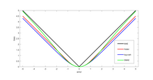
This function is quadratic for small values of a, and linear for large values, with equal values and slopes of the different sections at the two points where . The variable a often refers to the residuals, that is to the difference between the observed and predicted values , so the former can be expanded to[2]
The Huber loss is the convolution of the absolute value function with the rectangular function, scaled and translated. Thus it "smoothens out" the former's corner at the origin.

Motivation
[edit]Two very commonly used loss functions are the squared loss, , and the absolute loss, . The squared loss function results in an arithmetic mean-unbiased estimator, and the absolute-value loss function results in a median-unbiased estimator (in the one-dimensional case, and a geometric median-unbiased estimator for the multi-dimensional case). The squared loss has the disadvantage that it has the tendency to be dominated by outliers—when summing over a set of 's (as in ), the sample mean is influenced too much by a few particularly large -values when the distribution is heavy tailed: in terms of estimation theory, the asymptotic relative efficiency of the mean is poor for heavy-tailed distributions.
As defined above, the Huber loss function is strongly convex in a uniform neighborhood of its minimum ; at the boundary of this uniform neighborhood, the Huber loss function has a differentiable extension to an affine function at points and . These properties allow it to combine much of the sensitivity of the mean-unbiased, minimum-variance estimator of the mean (using the quadratic loss function) and the robustness of the median-unbiased estimator (using the absolute value function).
Pseudo-Huber loss function
[edit]The Pseudo-Huber loss function can be used as a smooth approximation of the Huber loss function. It combines the best properties of L2 squared loss and L1 absolute loss by being strongly convex when close to the target/minimum and less steep for extreme values. The scale at which the Pseudo-Huber loss function transitions from L2 loss for values close to the minimum to L1 loss for extreme values and the steepness at extreme values can be controlled by the value. The Pseudo-Huber loss function ensures that derivatives are continuous for all degrees. It is defined as[3][4]
As such, this function approximates for small values of , and approximates a straight line with slope for large values of .
While the above is the most common form, other smooth approximations of the Huber loss function also exist.[5]
Variant for classification
[edit]For classification purposes, a variant of the Huber loss called modified Huber is sometimes used. Given a prediction (a real-valued classifier score) and a true binary class label , the modified Huber loss is defined as[6]
The term is the hinge loss used by support vector machines; the quadratically smoothed hinge loss is a generalization of .[6]
Applications
[edit]The Huber loss function is used in robust statistics, M-estimation and additive modelling.[7]
See also
[edit]References
[edit]- ^ Huber, Peter J. (1964). "Robust Estimation of a Location Parameter". Annals of Statistics. 53 (1): 73–101. doi:10.1214/aoms/1177703732. JSTOR 2238020.
- ^ Hastie, Trevor; Tibshirani, Robert; Friedman, Jerome (2009). The Elements of Statistical Learning. p. 349. Archived from the original on 2015-01-26. Compared to Hastie et al., the loss is scaled by a factor of 1/2, to be consistent with Huber's original definition given earlier.
- ^ Charbonnier, P.; Blanc-Féraud, L.; Aubert, G.; Barlaud, M. (1997). "Deterministic edge-preserving regularization in computed imaging". IEEE Trans. Image Process. 6 (2): 298–311. Bibcode:1997ITIP....6..298C. CiteSeerX 10.1.1.64.7521. doi:10.1109/83.551699. PMID 18282924.
- ^ Hartley, R.; Zisserman, A. (2003). Multiple View Geometry in Computer Vision (2nd ed.). Cambridge University Press. p. 619. ISBN 978-0-521-54051-3.
- ^ Lange, K. (1990). "Convergence of Image Reconstruction Algorithms with Gibbs Smoothing". IEEE Trans. Med. Imaging. 9 (4): 439–446. doi:10.1109/42.61759. PMID 18222791.
- ^ a b Zhang, Tong (2004). Solving large scale linear prediction problems using stochastic gradient descent algorithms. ICML.
- ^ Friedman, J. H. (2001). "Greedy Function Approximation: A Gradient Boosting Machine". Annals of Statistics. 26 (5): 1189–1232. doi:10.1214/aos/1013203451. JSTOR 2699986.


