
File:Zipf's law on War and Peace.png

Original file (2,011 × 2,411 pixels, file size: 443 KB, MIME type: image/png)
| This is a file from the Wikimedia Commons. Information from its description page there is shown below. Commons is a freely licensed media file repository. You can help. |
Summary
| Description |
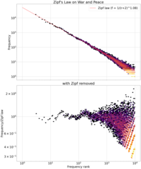
English: Zipf's Law on War and Peace, plotted according to "Zipf's word frequency law in natural language: A critical review and future directions" (ST Piantadosi, 2014).
It takes the text file, tokenizes it, then randomly split the tokens into two lists with 0.5 probability each. The word count in each list is counted. One word count is used to estimate the rank, and the other is used to estimate the frequency. This avoids the problem of correlated errors (see Piantadosi, 2014). The data is then plotted in log-log plot, and the Zipf law is fitted using the words with rank 10--1000 by least squares regression on the log-log plot. The alpha is estimated by hand (usually it's around 1 to 3) for convenience, though it can be estimated properly by standard least squares regression. The lower plot shows the remainder when the Zipf law is divided away. It shows that there is significant patterns not fitted by Zipf law. Text file of War and Peace from Project Gutenberg. Programmed in Python. Matplotlib codeimport nltk
import urllib.request
from collections import Counter
import matplotlib.pyplot as plt
import numpy as np
import re
import random
def zipf_plot(txt_url, title, alpha=1, gutenberg=True):
response = urllib.request.urlopen(txt_url)
print("response received")
long_txt = response.read().decode('utf8')
# Remove the Project Gutenberg boilerplate
if gutenberg:
pattern = r"\*\*\* START OF THE PROJECT GUTENBERG EBOOK [^\*]* \*\*\*"
match = re.search(pattern, long_txt)
if match:
start_index = match.end()
end_marker = "*** END OF THE PROJECT GUTENBERG EBOOK"
end_index = long_txt.find(end_marker, start_index)
long_txt = long_txt[start_index:end_index].strip()
else:
print("Pattern not found in the text.")
# Tokenize the text
tokenizer = nltk.tokenize.RegexpTokenizer('\w+')
tokens = tokenizer.tokenize(long_txt.lower())
# Randomly split the tokens into two corpora
random.shuffle(tokens)
half = len(tokens) // 2
corpus1, corpus2 = tokens[:half], tokens[half:]
# Count word frequencies in each corpus
counter1 = Counter(corpus1)
counter2 = Counter(corpus2)
# Find common words in both corpora
common_words = set(counter1.keys()) & set(counter2.keys())
# Create a dictionary of word, frequency pairs where frequency is the average of frequencies in two corpora
freqs = {word: (counter1[word] + counter2[word]) / 2 for word in common_words}
# Create a dictionary of word, rank pairs where rank is determined from the frequencies in the second corpus
ranks = {word: rank for rank, (word, freq) in enumerate(sorted([(w, counter2[w]) for w in common_words], key=lambda x: -x[1]), 1)}
# Create arrays for ranks and frequencies, ordered by rank
words = sorted(freqs.keys(), key=ranks.get)
ranks = np.array([ranks[word] for word in words])
counts = np.array([freqs[word] for word in words])
plt.rcParams.update({'font.size': 30})
fig = plt.figure(layout="constrained", figsize=(20, 24))
axes = fig.subplot_mosaic("A;B", sharex=True)
# Plot A: Zipf's Law with fitted line
ax = axes["A"]
ax.set_title(f"Zipf's Law on {title}")
ax.set_ylabel('Frequency')
# Zipf law fit
indices = (ranks >= 10) & (ranks <= 1000)
slope, intercept = np.polyfit(np.log(ranks[indices]), np.log(counts[indices]), 1)
ax.plot(ranks, np.exp(intercept) * ranks ** slope, color='red', alpha=1, label=f"Zipf law (f = 1/(r+{alpha})^{-slope:.2f})")
# Create the hexagonal heatmap using hexbin, on the log scale data
hb = ax.hexbin(ranks+alpha, counts, gridsize=100, cmap='inferno', bins='log', xscale='log', yscale='log')
# cb = plt.colorbar(hb, ax=ax)
# cb.set_label('log10(N)')
ax.legend()
ax.grid()
# Plot B: Zipf's Law with Zipf removed
ax = axes["B"]
ax.set_title("with Zipf removed")
ax.set_xlabel('Frequency rank')
ax.set_ylabel('Frequency/Zipf law')
# Create the hexagonal heatmap using hexbin, on the log scale data
hb = ax.hexbin(ranks+alpha, counts / (np.exp(intercept) * (ranks+alpha) ** slope), gridsize=100, cmap='inferno', bins='log', xscale='log', yscale='log')
# cb = plt.colorbar(hb, ax=ax)
# cb.set_label('log10(N)')
ax.legend()
ax.grid()
plt.show()
zipf_plot("https://www.gutenberg.org/cache/epub/2600/pg2600.txt", "War and Peace", alpha=2) |
| Date | |
| Source | Own work |
| Author | Cosmia Nebula |
Licensing
- You are free:
- to share – to copy, distribute and transmit the work
- to remix – to adapt the work
- Under the following conditions:
- attribution – You must give appropriate credit, provide a link to the license, and indicate if changes were made. You may do so in any reasonable manner, but not in any way that suggests the licensor endorses you or your use.
- share alike – If you remix, transform, or build upon the material, you must distribute your contributions under the same or compatible license as the original.
File history
Click on a date/time to view the file as it appeared at that time.
| Date/Time | Thumbnail | Dimensions | User | Comment | |
|---|---|---|---|---|---|
| current | 22:11, 11 July 2023 | | 2,011 × 2,411 (443 KB) | Cosmia Nebula | Uploaded while editing "Zipf's law" on en.wikipedia.org |
File usage
The following page uses this file: