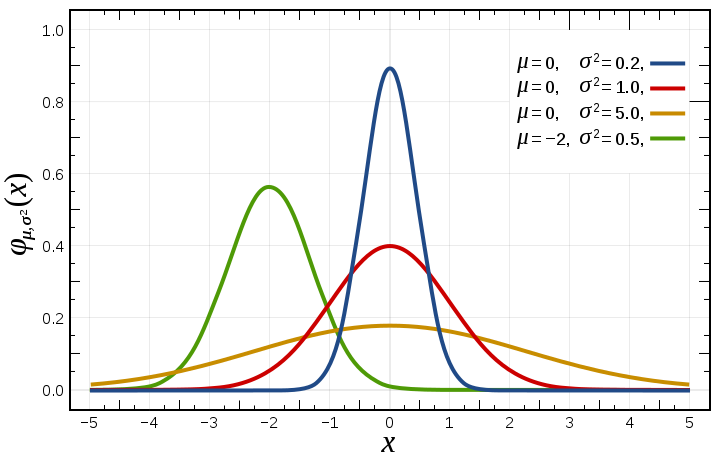
File:Normal Distribution PDF.svg
Appearance

Size of this PNG preview of this SVG file: 720 × 460 pixels. Other resolutions: 320 × 204 pixels | 640 × 409 pixels | 1,024 × 654 pixels | 1,280 × 818 pixels | 2,560 × 1,636 pixels.
Original file (SVG file, nominally 720 × 460 pixels, file size: 63 KB)
File history
Click on a date/time to view the file as it appeared at that time.
| Date/Time | Thumbnail | Dimensions | User | Comment | |
|---|---|---|---|---|---|
| current | 16:06, 29 April 2016 |  | 720 × 460 (63 KB) | Rayhem | Lighten background grid |
| 17:19, 22 September 2009 |  | 720 × 460 (65 KB) | Stpasha | Trying again, there seems to be a bug with previous upload… | |
| 17:15, 22 September 2009 |  | 720 × 460 (65 KB) | Stpasha | Curves are more distinguishable; numbers correctly rendered in roman style instead of italic | |
| 14:07, 27 June 2009 |  | 720 × 460 (55 KB) | Autiwa | fichier environ 2 fois moins gros. Purgé des définitions inutiles, et avec des plots optimisés au niveau du nombre de points. | |
| 18:22, 5 September 2008 |  | 720 × 460 (109 KB) | PatríciaR | from http://tools.wikimedia.pl/~beau/imgs/ (recovering lost file) | |
| 19:09, 2 April 2008 | No thumbnail | (109 KB) | Inductiveload | {{Information |Description=A selection of Normal Distribution Probability Density Functions (PDFs). Both the mean, ''μ'', and variance, ''σ²'', are varied. The key is given on the graph. |Source=self-made, Mathematica, Inkscape |Date=02/04/2008 |Author |
File usage
The following 13 pages use this file:
- Bell-shaped function
- Gaussian function
- Information geometry
- Normal distribution
- Probability distribution fitting
- User:Jlee4203/sandbox
- User:Minzastro/sandbox
- User:OneThousandTwentyFour/sandbox
- Wikipedia:Top 25 Report/September 16 to 22, 2018
- Template:Infobox probability distribution
- Template:Infobox probability distribution/doc
- Template:Infobox probability distribution/sandbox
- Template:Infobox probability distribution/testcases
Global file usage
The following other wikis use this file:
- Usage on ar.wikipedia.org
- Usage on az.wikipedia.org
- Usage on be-tarask.wikipedia.org
- Usage on be.wikipedia.org
- Usage on bg.wikipedia.org
- Usage on ca.wikipedia.org
- Usage on ckb.wikipedia.org
- Usage on cs.wikipedia.org
- Usage on cy.wikipedia.org
- Usage on de.wikipedia.org
- Usage on de.wikibooks.org
- Usage on de.wikiversity.org
- Usage on de.wiktionary.org
- Usage on en.wikibooks.org
- Usage on en.wikiquote.org
- Usage on en.wikiversity.org
- Usage on en.wiktionary.org
- Usage on eo.wikipedia.org
- Usage on es.wikipedia.org
- Usage on et.wikipedia.org
- Usage on eu.wikipedia.org
- Usage on fa.wikipedia.org
View more global usage of this file.
